Picture Books and Technical Papers

So I am a couple of weeks into a Grad. Dip. (Professional Writing) at University of Canberra…  My focus is on editing, which means one of my subjects is called Writing For Young People (?).

H in my alphabet.
H in my alphabet.

So far we’ve worked on ABC books, picture books, and children’s poems.

It’s a long way from diffuse scattering from organic molecular crystals, at least at first glance.  Writing for scientists who have PhDs and kids who can’t read is not as different as one might think.  The lecturer (Tony Eaton) has been very clear that in a picture book the words must not simply recapitulate the pictures, and that there needs to be a strong focus on the story and a willingness to pare away unnecessary detail, and to rephrase for clarity, and to collaborate and if necessary let the collaborator (illustrator, in the case of a picture book) represent ‘your’ ideas in ways you did not expect, and perhaps don’t even agree with; you need to be able to let go of the work.

When writing a paper I do expend some words drawing out the meaning of the figures, so there is a difference there, but the other exhortations do apply.  Precision is important.  Also, in both cases it helps to look at the work from a point of view not your own to make sure you have explained enough, but not too much.  And in science it is good to be dispassionate enough to let a collaborator reinterpret some data, criticise the reasoning, represent data in a different manner.  Both forms combine pictures and words in an attempt to be efficient and clear in their communication.

O is for ooze.
O is for ooze.

(I considered titling this posting ‘Blogger makes tenuous linkages in order to generate blog post’, but that applies to most of my entries anyway.)

Diffuseness.

Open Access in a Good Journal: A science publication at last!

I’ve had my rant about Open Access publishing, and now I’ve published in one.  Having said that, IUCrJ is the flagship open-access journal of the IUCr, the world peak body for crystallography, so it is rather different to being cold-called (well, emailed) by some recently established dodgy publisher.

The article, at  http://dx.doi.org/10.1107/S205225251402065X, is titled ‘Diffuse scattering and partial disorder in complex structures’. It was commissioned as part of the 2014 International Year of Crystallography, and I hope it outlines the history, state of the art, and value of the diffuse scattering technique, something I have talked about before, probably too much.  The main benefit of this one is the open access, which means that anyone can have a look at it.

Here’s a picture:

Paracetamol diffuse.
The 0kl layer of reciprocal space for one of the polymorphs of paracetamol, the common painkiller. An arbitrary, false-colour map of some diffuse scattering to add colour to a blog post.

Since the article is open access, I won’t write a whole lot about it, except to say that the historical part is mostly (entirely) the work of Richard Welberry, and I don’t think the history of this subfield has really be captured before by such an expert practitioner as he, so it is worth a read even if the more technical part of the article is of less interest.

It was written in LaTeX of course.


As if.

Short-Range Order in Ferroelectric Triglycine Sulphate

Jessica Hudspeth, now working hard at the ESRF, completed her PhD last year, and got it passed earlier this year.
In summary, she used diffuse x-ray and neutron scattering to look at the local ordering in triglycine sulphate, and learned some new and interesting information about the phase transition. The work shows that the use of diffuse scattering can reveal important new information even for materials that have been heavily studied using other techniques.

This is the abstract:

The short-range order in triglycine sulphate (TGS) was investigated using x-ray and neutron diffraction techniques. Complete deuteration of TGS was required for the neutron diffraction experiments and a new method was developed to grow single crystals of fully deuterated TGS by vapour diffusion crystallisation. The long-range structure of fully deuterated TGS was refined at several temperatures from single crystal neutron diffraction data and found to be consistent with the published structure of hydrogenous TGS. The phase transition temperature was
found to increase from about 322 K to about 334 K with complete deuteration.

The evolution of the long-range structure with temperature was investigated using x-ray and neutron powder diffraction. All of the lattice parameters hada single cusp at the phase transition, except for the b lattice parameter, which also had a second cusp about 34 K below TC. In contrast to the lattice parameter behaviour, the unit cell volume was found to increase monotonically with temperature. The length of the hydrogen bonds between the disordered N atom on glycine 1 (G1) and the surrounding molecules was found to increase with temperature, whereas the length of the short hydrogen bond between G2 and G3 decreased slightly with temperature. This supports the suggestion that weakening of the hydrogen bonds decouples G1 from G2 and G3, allowing the system to become disordered. Except around the ferroelectric to paraelectric phase transition temperature, no abnormalities in the behaviour of any of the refined parameters were observed, suggesting that TGS only has a single phase transition.

The short-range order in TGS was investigated by collecting single crystal x-ray and neutron diffuse scattering at several temperatures from well below to well above TC. Well below TC, the diffuse scattering was purely thermal diffuse scattering due to correlations of the atomic  displacements. Close to the phase transition, diffuse streaks perpendicular to b∗ were also present in the diffuse scattering patterns, which were due to short-range order of the G1 orientations parallel to the ferroelectric b axis. The onset of significant short-range order appears to occur about 40 K below TC. The correlations are strongest at the phase transition and then decrease with temperature above TC.

The short-range order was modelled using a combination of a displacive disorder and an orientational disorder Monte Carlo simulation. The intermolecular interactions that give rise to correlated atomic displacements were modelled by treating them like Hooke’s law springs. The force constants for the interactions were parameterised in a number of ways, the most successful of which was an empirical formula developed by Chan et al.

The short-range order of the G1 orientations was modelled using an Ising-type model. The G1 interactions that lead to short-range order along the ferroelectric b-axis appear to be mediated by the short hydrogen bond between G2 and G3. This suggests that the hydrogen bonding, rather than the dipole-dipole interactions, plays the dominant role in the ferroelectric ordering of TGS. While the hydrogen bonding gives rise to strongly correlated chains of G1 molecules along b, it is likely that there are also weaker correlations between the chains due to dipole-dipole
interactions. This provides a mechanism for TGS to go from short-range ordered in 1-dimension, to long-range ordered in 3-dimensions as it is cooled through TC.


And here’s a picture (HTGS means hydrogenous, as distinct from deuterated):

tgs

The Smallest Possible Contribution

The very excellent @minutephysics just put out a video on the ‘everywhere stretch’, otherwise known as the Big Bang.  It needed a small diagram, generated via LaTeX, and it ended up being provided by me.  It appears for about 0.04 seconds of the 5 minute presentation and it looks like this:

proj_1

By my calculation, if every 0.04 seconds of the video took as much time as I took for the diagram, the video would require about two months non-stop work to make.  Clearly we don’t enough appreciate the free content that Henry and his colleagues provide for us!

It also was a nice example for me of how so-called ‘social media’ allows people to connect by interest and not accidents of geography.

Technical details:

I should have but did not use some clever LaTeX package for drawing this diagram.  I drew it using xFig, exported to a LaTeX picture environment and edited the output by hand to make the equations come out right.  Took 5 or 10 minutes and the code looks like this (embedded in a .tex file so that it can be compiled for test purposes):


\documentclass{article}
\usepackage{color}
\begin{document}
\setlength{\unitlength}{4144sp}%
%
\begingroup\makeatletter\ifx\SetFigFontNFSS\undefined%
\gdef\SetFigFontNFSS#1#2#3#4#5{%
\reset@font\fontsize{#1}{#2pt}%
\fontfamily{#3}\fontseries{#4}\fontshape{#5}%
\selectfont}%
\fi\endgroup%
\begin{picture}(1332,1557)(3136,-3730)
\thinlines
{\color[rgb]{0,0,0}\put(3556,-2581){\vector( 0,-1){810}}
}%
{\color[rgb]{0,0,0}\put(3826,-2446){\vector( 1, 0){495}}
}%
{\color[rgb]{0,0,0}\put(4456,-2671){\vector(-1,-1){697.500}}
}%
\put(3421,-3661){\makebox(0,0)[lb]{\smash{{\SetFigFontNFSS{12}{14.4}{\familydefault}{\mddefault}{\updefault}{\color[rgb]{0,0,0}$U$}%
}}}}
\put(3381,-3031){\makebox(0,0)[lb]{\smash{{\SetFigFontNFSS{12}{14.4}{\familydefault}{\mddefault}{\updefault}{\color[rgb]{0,0,0}$\pi$}%
}}}}
\put(4366,-2491){\makebox(0,0)[lb]{\smash{{\SetFigFontNFSS{12}{14.4}{\familydefault}{\mddefault}{\updefault}{\color[rgb]{0,0,0}$U \times F$}%
}}}}
\put(4276,-3121){\makebox(0,0)[lb]{\smash{{\SetFigFontNFSS{12}{14.4}{\familydefault}{\mddefault}{\updefault}{\color[rgb]{0,0,0}$\textrm{proj}_1$}%
}}}}
\put(3151,-2446){\makebox(0,0)[lb]{\smash{{\SetFigFontNFSS{12}{14.4}{\familydefault}{\mddefault}{\updefault}{\color[rgb]{0,0,0}$\pi^{-1}(U)$}%
}}}}
\put(4001,-2356){\makebox(0,0)[lb]{\smash{{\SetFigFontNFSS{12}{14.4}{\familydefault}{\mddefault}{\updefault}{\color[rgb]{0,0,0}$\phi$}%
}}}}
\end{picture}%

\end{document}

A Long Long Time Ago…Part 4

As noted recently, rather too many years ago I wrote a thing called ‘THE COMPLETE HISTORY OF SCIENCE: REVISED, UPDATED AND GENERALLY REFURBISHED’ and it saw the light of day, so to speak, in The Mentor, an Australian fanzine. Below is part 4.  Part 2 is here. Part 3 I leave to the imagination.

THE COMPLETE HISTORY OF SCIENCE: REVISED, UPDATED AND GENERALLY REFURBISHED.

Part IIII (also known as Part IV)


Isaac Newton: The year Galileo died, Isaac Newton was born. A year later, he had his first birthday, establishing a pattern which was to remain with him all his life. Isaac Newton  is best known for three things: Inventing calculus, making up his three laws (thus revealing Kepler’s influence), and inventing apples. He therefore opened a rift between science and religion, as the Church insisted that the apple had been invented by the snake – a dubious proposition indeed.
The discovery of the apple was of considerable gravity. Newton thus called it his theory of apple gravity, though this is generally shortened to the theory of gravity, a meaningless contraction. In the theory, the attractive force between two masses is inversely proportional to their separation squared and proportional to whether one of them is ripe or not. Newton’s greatest leap was to say that this ‘apple force’ also acted upon the moon and other celestial bodies, allowing us to conclude that the moon itself is an apple – presumably very old and, therefore, wrinkly and discoloured.
His three laws were all to do with force. The third one (the important one) states that for every action there is an equal and opposite reaction, a principle that rears its head in business and politics as well as physics.
Newton, however, was also an alchemist. This is a black mark against him. When added to all the extra work that high school students have to do because of him, it becomes doubtful whether he was, after all, a benefactor of mankind.
Lastly, Newton set the trend of having a measurement named after him – the Newton, the unit of force. This is nothing like the ‘Nightstick’, which is the unit of ‘Brute Force’.

Edmund Halley: Edmund Halley was a friend of Newton’s. His invention of comets (“hairy stars”) was a breakthrough. So much so that one was named after him – though comet Edmund was never seen again.

Leibniz: Though less famous than Newton, Leibniz was still famous enough to also invent calculus.

After Newton: After a flurry of activity, science slowed down for a while due to a lack of historically notable figures. Britain in particular suffered, since they’d been letting Newton do all the science and he was dead. In America, Benjamin Franklin connected himself to lighting via a kite. Simultaneously, he: 1) Proved that lighting was a form of electricity and; 2) Invented the ‘perm’ hairstyle.
In Europe things soon picked up again. Mathematics was very popular. In particular, a Frenchman called Lagrange formulated the principle of least action. Like Newton’s third law, this also has been co-opted by politicians.
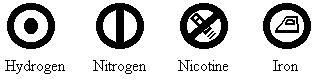
Great strides were made by the chemist John Dalton. He is, however, best known for his chemistry, in which he resurrected the ancient Greek idea of the ‘atom’. He also invented symbols for each kind of atom:

daltonThough his framework has remained largely intact, a number of his identifications have been called into question. And the proposal of naming an element ‘Dolt’ in his honour has floundered.
But it was good to have atoms, because now people had something to be made of. Also, it would give all those atomic scientists something to do during World War II.

After Dalton came his children. In science also things were picking up. The publication of Frankenstein, by Mary Shelley, gave great impetus to biology (and the odd corpse), and Gregor Mendel (a monk) invented genetics, something which gave all sorts of people excuses for being the sort of people they were.

Faraday & Maxwell etc: Inextricably linked in the history of science are the names Farawell and Maxaday, who between them invented electromagnetism.

There was a lot of quantifying going on. Wellday and Faramax quantified electricity, Mendeleyev quantified the elements, and Arthur Waddington-Smith quantified garden gnomes, though this is sometimes seen as a lesser achievement.

Charles Darwin: No figure stands taller in the annals of nineteenth century science than Charles Darwin, father of evolution. Above all scientists, he really got up God’s nose. His proposal that mankind and the apes had a common ancestor – whom he tentatively dubbed ‘Hubert’ – gave many cause for alarm, all the more when he revealed that a beagle had given him the idea. However, he received quite a bit of support from the wives of boorish men, as these ladies found that his theory dovetailed nicely with their own observations.

Darwin wrote two great books. The Origin of Species, in which he explained evolution, and The Descent of Man, in which he described man’s descent from noble savage to tax collector. Objections came from all directions, generally from people denying that they were related to tax collectors.

Edison: Meanwhile, in America Thomas Edison was busy inventing the twentieth century. He was in a bit of a hurry, since he was working to a deadline. Amongst his inventions were the electric light, the phonograph, and the Spud-O-Matic, though the latter never really took off.

So at the End of the Nineteenth Century: So at the end of the nineteenth century, they thought they knew it all. Newton had worked out Newton’s Laws, Maxwell had worked out Faraday’s Equations, Mendel had worked out Mendel’s Rules, Darwin had worked out Darwin’s Theory, and Alfred Nobel was making things blow up and giving out prizes.
But then the Universe started obeying quantum mechanics, and all that went out the window.

Magnetic structure and glassiness in…

So, the latest paper to come out is ‘Magnetic structure and glassiness in Fe0.5Ni0.5PS3‘, in Journal of Magnetism and Magnetic Materials 334 (2013) 82–86 (http://dx.doi.org/10.1016/j.jmmm.2013.01.023).

The science is I think interesting.  We find that by mixing Ni and Fe on the metal site we induce a time-dependence in the magnetic behaviour. That is to say that the system likes to order antiferromagnetically, with the magnetic moments on the metal sites cancelling each other out, but that this ordering is quite slow. It takes hours for the magnetic moments to reach their final arrangement.

This shows up in the magnetic susceptibility in the way that the susceptibility — how strongly the material reacts to an applied magnetic field, basically — depends on whether you are warming the sample up or cooling it down.  The picture below shows that — as we heat up the cusp in the (admittedly noisy) data comes in at about 140K, but on cooling it comes in at about 90K.  So as we cool down from the paramagnetic high temperature state, the system remains paramagnetic till 90K, where if we heat up from the low temperature magnetically ordered state, the system stays ordered up to 140K.  If we are cooling and we get to, say, 100K then stop cooling and just measure as a function of time, we get a nice stretched exponential decay of the magnetisation until it reaches the value it would have on the lower curve.  that is, it follows the red line, and take about three hours to get there.  That means that the lower curve — what we measure on heating — is measuring the true equilibrium state.

Magnetic susceptibility
Magnetic susceptibility of Fe0.5Ni0.5PS3 as a function of temperature.

One of the other nice things about this paper is that two of the authors — S. Brazier-Hollins and D.R. James — were project students rather than full academics or Ph.D. scholars. Their work on the project was enthusiastic and of high quality, and it was really nice to pull a range of disparate contributions together and see it in print.